Clarifing a misunderstanding of back-propagation through time method

1. INTRODUCTION

Back-propagation through time (BPTT) algorithm is a gradient training strategy for recurrent neural network, and was first proposed by Rumelhart et al. (1986).

2. BACK-PROPAGATION THROUGH TIME (BPTT) ALGORITHM

For a stardand recurrent neural network (RNN) model (as showed in Figure 1), it can be represented as:

$\begin{align*} &s_t = f(Ux_t + Ws_{t-1})\\ &y_t = Vs_t \end{align*}$

Figure 2. Architecure of recurrent nerual network language models

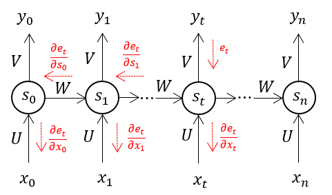
At time setp $t$ , let the error in output layer are $e_t$ , ( $0\leq{t}\leq{n}$ ). Using BPTT algorithm with out any truncation, the error $e_t$ will be backpropagation throgh all the previous step (Figure 2). Take $x_i$ ( $0\leq{i}\leq{t}$ ) as an example, the error gradient is:

$\frac{\partial{e_t}}{\partial{x_i}}=\frac{\partial{e_t}}{\partial{s_i}}\frac{\partial{s_i}}{\partial{x_i}}$

Figure 2. Back-propagate errors using bptt

the final error gradient for $x_i$ is

$\frac{\partial{E_i}}{\partial{x_i}}=\sum_{t=i}^{n}\frac{\partial{e_t}}{\partial{x_i}}$

One common way to implement bptt is showed as following code block which is written in Python. At each time step, the error should be back-propagated throngh all the previous time steps. If the input sequence is long, the computation will be very expensive. This sometimes is taken as the reason for why truncation needed for BPTT by mistake.

def bptt(dLds):
    """A naive implementation of BPTT.
    """
    T = len(dLds)
    dLdb = np.zeros(hidden_size)
    dLdx = np.zeros((T, input_size))
    dLdU = np.zeros((hidden_size, input_size))
    dLdW = np.zeros((hidden_size, hidden_size))
    for t in xrange(T-1, -1, -1):
        dLdp = dLds[t] * (1.0 - (s[t] ** 2))
        for step in xrange(t, -1, -1):
            dLdU += np.outer(dLdp, x[step])
            dLdW += np.outer(dLdp, s[step-1])
            dLdx[step] += np.dot(self.U.T, dLdp)
            dLdb += dLdp
            dLdp = np.dot(W.T, dLdp) * (1.0 - (s[step-1] ** 2))
    return dLdx, dLdU, dLdW, dLdb

It is a common misunderstanding of BPTT. At each time step, it is not necessary to back-propagate the error throught all previous steps immediately. When training recurrent neural network, BPTT is only applied in hidden layer and input layer, and, with a careful observation, the error gradient for parameters in hidden layer and input layer can be decomposed into two parts, i.e., the error from current output and the error from all late time step:

$\begin{align*} \frac{\partial{E_i}}{\partial{x_i}}&=\sum_{t=i}^{n}\frac{\partial{e_t}}{\partial{x_i}}=\frac{\partial{s_i}}{\partial{x_i}}\sum_{t=i}^{n}\frac{\partial{e_t}}{\partial{s_i}}\\ &=U^T\frac{\partial{e_i}}{\partial{s_i}} + U^TW^T\frac{\partial{E_{i+1}}}{\partial{s_i}} \end{align*}$

With dynamic planning, instead of propagating the error to all the previous time step immediately, just calculate the error gradients for each hidden layer firstly and accumulate the error gradient to the hidden state of directly previous step at each time step. The code for this implementaion of BPTT in python is as follows:

def new_bptt(dLds):
    """A optimized implementation of BPTT.
    """
    dLdb = np.zeros(hidden_size)
    dLdx = np.zeros((T, input_size))
    dLdU = np.zeros((hidden_size, input_size))
    dLdW = np.zeros((hidden_size, hidden_size))
    for t in xrange(T-1, -1, -1):
        dLdp = dLds[t] * (1.0 - (s[t] ** 2))
        dLdU += np.outer(dLdp, x[t])
        dLdW += np.outer(dLdp, s[t-1])
        dLdx[t] += np.dot(self.U.T, dLdp)
        dLdb += dLdp
        self.dLds[t-1] += np.dot(W.T, dLdp)
    return dLdx, dLdU, dLdW, dLdb

For training recurrent network models on short sequences, truncation is not necessary. Take recurrent neural language model as an example, if treat data set as individual sentences and training model sentence by sentence, no truncation need to be applied. On the other hand, if data set is dealt with as a single long sequence, it is not feasible to do a complete back-propagation and the convergence will be diffcult if the model is updated after running over the whole long sequence. In this case, update block is usually adopted and the model is updated each block (details about this please refer to previous post). The errors in current block will be back-propagated only several time steps in previous blocks, this is truncated BPTT.