The source code for the neural network language models described in this post are implemented using both python and C++.
1. INTRODUCTION
Generally, well designed language model makes a critical difference in various natural language processing (NLP) tasks, including speech recognition, machine translation, semantic extraction and etc. Language modeling (LM), therefore, has been the research focus in NLP field all the time, and a large number of sound research results have been published for decades. N-gram based language modeling, a non-paramtric approach, is used to be state of the art, but now a paramtric approach - neural network language modeling (NNLM) is considered to show the best performance, and become the most commonly used LM technique in multiple NLP tasks.
Although some previous attempts, details on which are provided by Schwenk (2007), had been made to introduce artificial neural network (ANN) into LM, NNLM began to attract researches’ attention only after Bengio et al. (2001, 2003), and did not show prominent advantage over other techniques of NNLM until recurrent neural network (RNN) was investigated for LM (Mikolov et al., 2010, 2011). After more than a decade’s research, there are numerous imporvements, marginal or critical, over basic NNLM have been proposed. In this post, the basic neural network language models will be described, and the improvement techniques will be introduced in following posts.
2. NEURAL NETWORK LANGUAGE MODELS, NNLMs
The goal of statistical language models is to estimate the probability of a word sequence $w_1w_2…w_T$ in a natural language, and the probability can be represented by the production of the conditional probability of each word given all the previous ones:
where, $w_{i}^{j}\;=\;w_iw_{i+1}\dots{w_{j-1}w_j}$. This chain rule is established on the assumption that the word in a sequence only depend on its prvious context, and forms fundation of all statistical language modeling. NNLM is a kind of statistical language modeling, so it is also termed as neural probabilistic lanuage modeling or neural statistical lanuage modeling, and the objective of NNLM is to learn the conditional probability function of words. According to the adopted artificial neural network, neural network language model can be classified as: feed-forward neural network language model (FNNLM), recurrent neural network language model (RNNLM) and long short term memory (LSTM) recurrent neural network language model (LSTM-RNNLM).
2.1. Feedforward Neural Network Language Model, FNNLM
As metioned above, the objective of FNNLM is to evaluate the conditional probability $P(w_t{\mid}w_{1}^{t-1})$, but FNNLM lacks of an effective way to represent history context. Hence, the idea of n-gram model is adopted in FNNLM that words in a word sequence more statistically depend on the words closer to them, and only the $n-1$ direct predecessor words are condsidered when evaluating the conditional probability, this is:
The architecture of the original FNNLM in Bengio et al. (2003) is showed in Figure 1, and $w_0$, $w_{T+1}$ are start and end marks of word sequence respectively. In this model, a vocabulary is pre-built from a training data set, and each word in this vocabulary is assigned with a unique index. To predict the conditional probabiltiy of word $w_t$, its direct previous words $w_{t-n+1},…,w_{t-1}$ are projected linearly into feature vectors using a shared matrix $C\in{\mathbb{R}^{k\times{m}}}$ according to their index in vocabulary, where $k$ is the size of the vocabulary and $m$ is the feature vectors’ size. In fact, each row of projection maxtrix $C$ is a feature vector of a word. The input $x\in\mathbb{R}^{n_i}$ of FNNLM is formed by concatenating the feacture vectors of words $w_{t-n+1},…,w_{t-1}$, where $n_i=m\times(n-1)$ is the size of FNNLM’s input layer. The feedforward neural network model can be generally repesented as:
Where, $U\in\mathbb{R}^{n_h\times{n_i}}$, $V\in\mathbb{R}^{n_o\times{n_h}}$ are weight matrixes, $n_h$ is the size of hidden layer, $n_o=k$ is the size of output layer, weight matrix $M\in\mathbb{R}^{n_o\times{n_i}}$ is for the direct connections between input layer and output layer, $b\in\mathbb{R}^{n_h}$ and $d\in\mathbb{R}^{n_o}$ are bias vectors in hidden layer and output layer respectively, $y\in\mathbb{R}^{n_o}$ is output vector, and $f(\cdot)$ is activation function.
The $i$-th element of output vector $y$ is the unnormalized coditional probability for the word with index $i$ in vocabulary. In order to guarantee all the output probailities positive and summing to 1, a softmax layer is always adopted following the output layer of feedforward nerual network:
where $y(w_i,w_{t-n+1}^{t-1})\;(i\;=\; 1, 2, …,k)$ is the $i$-th element of ouput vector $y$.
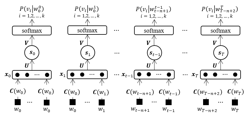
Figure 1. Architecure of feed-forward nerual network language models
In Bengio’s initial work (Bengio et al., 2001), two different architetures of FNNLM are proposed: direct and cycling architecture. The direct architeture model has been described above. In cycling architecture model, the input of model is the concatenation of feature vectors of both words in history context and candidate next word. For a given history context $w_{t-n+1}^{t-1}$, each word $w_{i} (i=1, 2, \dots, k)$ in vocabulary will be taken as a candidate next word, and its conditional probability is evaluated by FNNLM. The output of model is a scalar $y(w_{i},w_{t-n+1}^{t-1})$ instead of a vector which is the unnormalized conditioanal probability for the corresponding candidate next word $w_{i}$. Again, the outputs of all candidate next words are normalized using a softmax function. The experimental results in Bengio et al. (2001)) show that the direct architecture model is about 2% better than the cycling one, and direct architecture is adopted in all following neural network language models.
Training of neural network language models is achieved by maximizing the log-likelihood of the training data:
where, is the set of model’s parameters of NNLMs to be trained, is a regularization term.
The recommended learning algorithm for neural network language models is stochastic gradient descent (SGD) method using backpropagation (BP) algorithm. A commonly used loss function for training neural network language models is corss-entropy:
where, $\hat{o}$ is the desired outputs, and $o$ is the outputs of neural network language models, i.e., the outputs of softmax layer. Because the desired outputs $\hat{o}$ are all one-hot vectors, this loss function can be simplified as:
where, $i$ is the index of target word. The gradient for the outputs $y_i, i=1,2,\dots,k$ of neural network model at step is:
The log-likehood gradient for all outputs can be represented as:
then, the log-likehood gradient for parameters set $\theta$ is:
The parameters are updated as:
where, is learning rate and is regularization parameter.
The performance of neural network language models is usually measured by perflexity (PPL) which can be defined as:
Perflexity can be defined as the exponential of the average number of bits required to encode the test data using a language model and lower perflexity indicates that the language model is closer to the true model which generates the test data.
2.2. Recurrent Neural Network Language Model, RNNLM
The idea of applying RNN in LM was proposed much earlier (Bengio et al., 2003; Castro and Prat, 2003), but the fisrt serious attempt to build a RNNLM was made by Mikolov et al. (2010, 2011). RNNs are fundamentally different from feedforward architecture in the sense that they not only operate on an input space but also on an internal state space, and the state space enables the representation of sequentially extended dependencies. Therefore, arbitrary length of word sequence can be dealt with using RNNLM, and all previous context can be taken into account when predicting next word. As showed in Figure 2, the representation of words in RNNLM is the same as that of FNNLM, but the input of recurrent neural network at each step is the feature vector of a direct preivous word instead of the concatenation of the $n-1$ previous words’ feature vectors and all other previous words are taken into account by the internal state of previous step. At step $t$, recurrent neural network can be described as:
where, weight matrix . Tand its size of input layer $n_i=m$. The output of recurrent neural network are also unnormalized probabilities and should be regularized by a softmax layer.

Figure 2. Architecure of recurrent nerual network language models
Because of the involvement of previous internal state at each step, back-propagation through time (BPTT) algorithm Rumelhart et al. (1986) is prefered for better performance when training RNNLMs. If data set is treated as a single long word sequence, truncated BPTT shoud be used and Mikolov (2012)) reports that back-propagating error gradients through 5 steps is enough, at least for small corpus. If data set is dealt with sentence by sentence, the error gradient can be back-propagated trough each whole sentence without any truncation.
2.3 LSTM Neural Network Language Model, LSTM-NNLM
Although RNNLM can deal with all of the predecessor words to predict next word in a word sequence, but it is quit difficult to train over long term dependencies because of the vanishing problem (S. Hochreiter and J. Schmidhuber, 1997). This problem can be addressed by using Long-Short Term Memoery (LSTM) neural network, and LSTM neural network was introduced to LM by Sundermeyer et al. (2013). LSTM-NNLM is almost the same as RNNLM, the only difference is the architecture of neural network. LSTM neural network was proposed by Schmidhuber (1997) and was refined and popularized in following works (Gers and Schmidhuber, 2000; Cho et al. 2014). The general architecture of LSTM neural network is:
Where, , , are input gate, forget gate and output gate, respectively. is previous state of nodes. , , , , , , , , , , , are all weight matrixes. , , , , and are bias vectors. is the activation function in hidden layer and is the activation function for gates.
3. COMPARISON OF NNLMS WITH DIFFERENT ARCHITECTURES
Comparision among different neural network language models have already been made on both small and large corpus (Mikolov, 2012; Sundermeyer et al., 2013). The results show that, generally, RNNLM outperform FNNLM and the best performance is achieved using LSTM-NNLM. However, the neural network language models in these researches are optimized using various techniques, even combined with other kind language models, let alone the different experimental setups and implementation details, which make the comparison results failed to illustrate the fundamental discrepancy in the performance of neural network language models. Here, comparative experiment on neural network language models with different architecture are repeated on Brown Corpus. The models in these experiments were all implemented plainly, and only a class-based speed-up technique was used which will be introduced later. Experiments were performed on the Brown Corpus, and the experimental setup for Brown corpus is the same as in Bengio et al. (2003), the first 800000 words (ca01$\sim$cj54) were used for training, the following 200000 words (cj55$\sim$cm06) for validation and the rest (cn01$\sim$cr09) for test.
Table 1. Comparison of different NNLMs
| Models | Direct | Bias | Brown | |||
|---|---|---|---|---|---|---|
| FNNLM | 5 | 200 | 200 | No | No | 223.85 |
| RNNLM | - | 200 | 200 | No | No | 221.10 |
| LSTMLM | - | 200 | 200 | No | No | 237.93 |
| LSTMLM | - | 200 | 200 | Yes | No | 242.54 |
| LSTMLM | - | 200 | 200 | No | Yes | 237.18 |
The experiment results are showed in Table 1 which suggest that, on a small corpus likes Brown Corpus, RNNLM and LSTM-RNN did not show a remarkable advantage over FNNLM, instead a bit higher perplexity was achieved by LSTM-RNNLM. Maybe more data is needed to train RNNLM and LSTM-RNN because more previous context are taken into account by RNNLM and LSTM-RNNLM when predicting next word. LSTM-RNNLM with bias terms or direct connections was also evaluated. With direct connections, a slightly higher perpleixty but shorter training time was obtained. An explanation given by Bengio et al. (2003) is that direct connections provide a bit more capacity and faster learning of the “linear” part of mapping from inputs to outputs but impose a negative effect on generalization. For the bias terms, no significant improvement of performance was gained which was also observed on RNNLM by Mikolov, 2012.


